Linear Mixed Effects Models

Modelling data from an RCT examining digital interventions for depression, alcohol use, suicide risk, and loneliness in older adults

code migration in process

Introduction

In this analysis, we examine the efficacy of two eHealth interventions designed to improve co-ocurring depression and alcohol misuse in older Australians (60+).

We examined:

1. Whether access to an online clinician moderated peer support platform alone improves depression, alcohol use, and suicidality in Australians over 60 (Breathing Space group)
2. Whether access to a structured, evidence-based, web-delivered congitive behavioural therapy program, in addition to Breathing Space, enhances these outcomes beyond social networking alone (SHADE+ group)
3. Whether the Breathing Space social network improves social isolation in Australians 60+

Outcome Descriptives

# create function for creating an outcome table

make_outcome_block <- function(data, outcome_var, outcome_label) {
  # convert outcome_var to a symbol so we can use !!
  outcome_var <- rlang::ensym(outcome_var)

  # summarise outcome by time and group (numeric means/sds)
  long <- data |>
    select(group, event, value = !!outcome_var) |>
    mutate(
      time = case_when(
        event == 0 ~ "Baseline",
        event == 12 ~ "12-weeks",
        event == 26 ~ "26-weeks",
        TRUE ~ as.character(event)
      ),
      time = factor(
        time,
        levels = c("Baseline", "12-weeks", "26-weeks"),
        ordered = TRUE
      )
    ) |>
    filter(!is.na(value)) |>
    group_by(group, time) |>
    summarise(
      mean = mean(value, na.rm = TRUE),
      sd = sd(value, na.rm = TRUE),
      .groups = "drop"
    )

  # numeric means wide by time (for deltas)
  mean_wide <- long |>
    select(group, time, mean) |>
    tidyr::pivot_wider(
      id_cols = group,
      names_from = time,
      values_from = mean,
      names_glue = "{time}_mean"
    )

  # ensure all time columns exist, even if NA
  for (tn in c("Baseline_mean", "12-weeks_mean", "26-weeks_mean")) {
    if (!tn %in% names(mean_wide)) mean_wide[[tn]] <- NA_real_
  }

  mean_wide <- mean_wide |>
    mutate(
      delta = `26-weeks_mean` - `Baseline_mean`
    )

  # formatted mean (SD) wide by time
  cell_wide <- long |>
    mutate(
      mean = round(mean, 1),
      sd = round(sd, 1),
      cell = sprintf("%.1f (%.1f)", mean, sd)
    ) |>
    select(group, time, cell) |>
    tidyr::pivot_wider(
      id_cols = group,
      names_from = time,
      values_from = cell,
      names_glue = "{time}_cell"
    )

  # ensure all formatted time columns exist
  for (tn in c("Baseline_cell", "12-weeks_cell", "26-weeks_cell")) {
    if (!tn %in% names(cell_wide)) cell_wide[[tn]] <- NA_character_
  }

  # merge numeric and formatted,
  full <- mean_wide |>
    left_join(cell_wide, by = "group") |>
    mutate(
      delta_str = ifelse(
        is.na(delta),
        NA_character_,
        sprintf("%.1f", round(delta, 1))
      )
    ) |>
    transmute(
      Label = as.character(group),
      Baseline = `Baseline_cell`,
      `12-weeks` = `12-weeks_cell`,
      `26-weeks` = `26-weeks_cell`,
      `Δ 26w – baseline` = delta_str
    )

  # add outcome header row on top
  header_row <- full[0, , drop = FALSE]
  header_row[1, ] <- NA_character_
  header_row$Label[1] <- outcome_label

  tab <- bind_rows(header_row, full)

  # force all columns to character to bind_rows across outcomes
  tab[] <- lapply(tab, as.character)

  tab
}

# apply function to outcomes

# create table
out_table <- bind_rows(
  make_outcome_block(df, gds_score_new, "Depression (GDS-SF)"),
  make_outcome_block(df, smast_score_new, "Alcohol use (SMAST-G)"),
  make_outcome_block(df, sidas_score, "Suicide Risk (SIDAS)"),
  make_outcome_block(df, lonely_total, "Loneliness (UCLA Loneliness Scale)")
)

out_table <- out_table |>
  mutate(across(everything(), ~ ifelse(is.na(.), "", .)))

# create list of outcome labels
outcome_labels <- c(
  "Depression (GDS-SF)",
  "Alcohol use (SMAST-G)",
  "Suicide Risk (SIDAS)",
  "Loneliness (UCLA Loneliness Scale)"
)

out_table <- out_table |>
  flextable() |>
  my_flextable() |> 
  padding(i=c(2:3, 5:6, 8:9, 11:12), j=1, padding.left=20) |> 
  set_header_labels(Label = "Outcome") |> 
  align(j = c(2:5), part = "all", align = "center")

out_table

Table 1: Mean (SD) at each timepoint and change from baseline to 26 weeks for depression, alcohol use, suicide risk, and loneliness by treatment group

Outcome	Baseline	12-weeks	26-weeks	Δ 26w – baseline
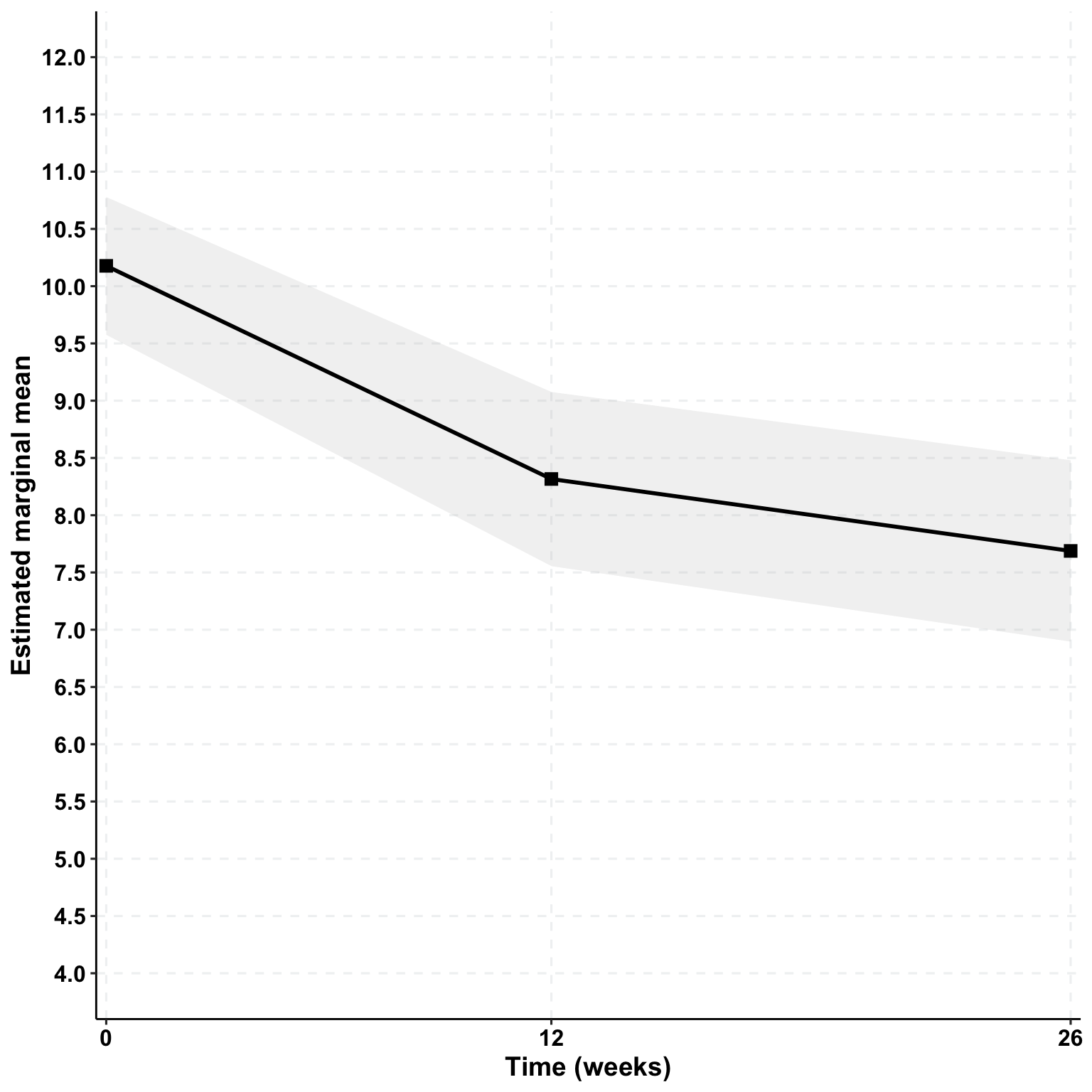
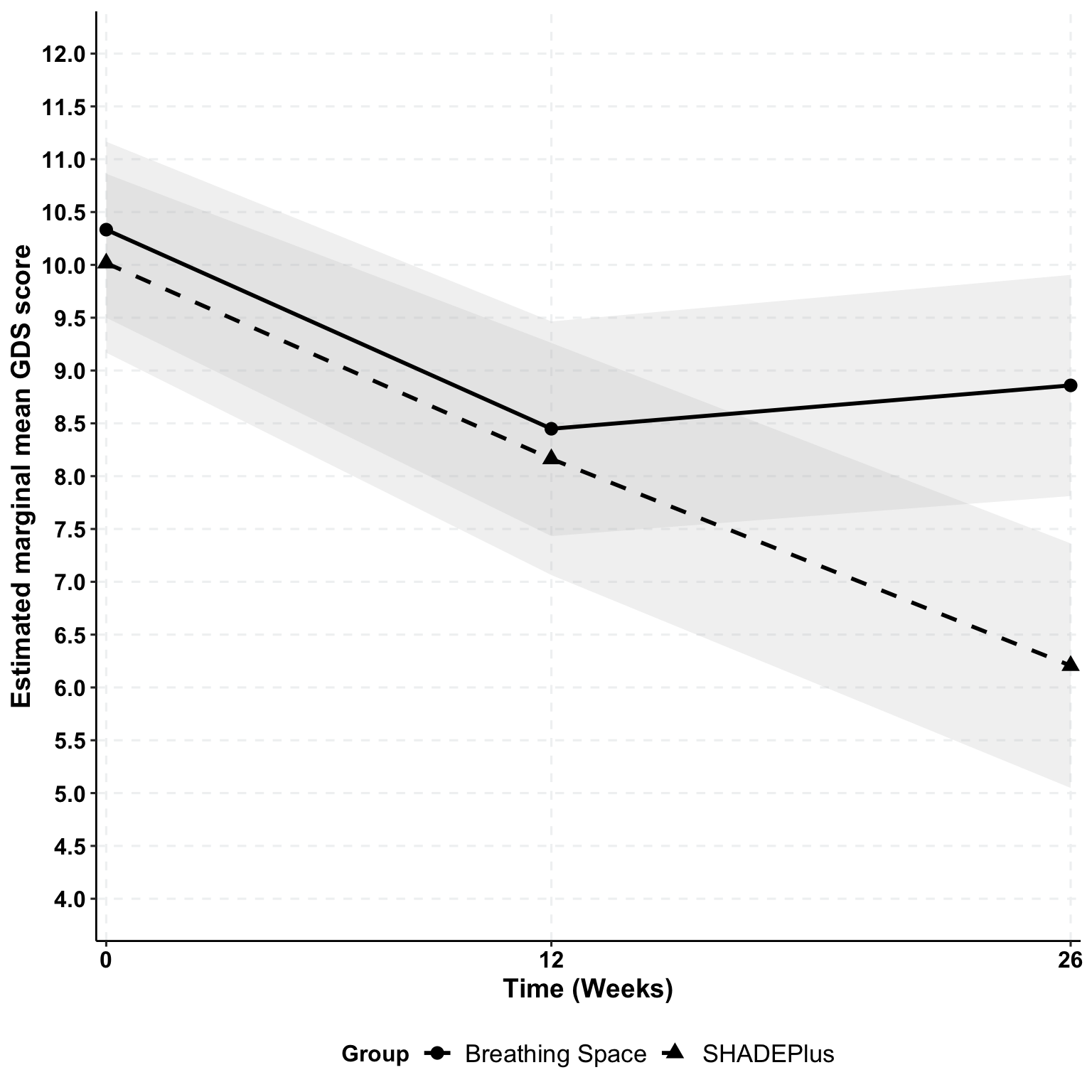
Depression (GDS-SF)
Breathing Space	10.3 (2.9)	8.3 (3.7)	8.8 (4.1)	-1.5
SHADEPlus	10.0 (2.9)	8.1 (3.8)	6.1 (4.2)	-3.9
Alcohol use (SMAST-G)
Breathing Space	6.4 (2.2)	5.6 (2.4)	5.7 (2.4)	-0.7
SHADEPlus	6.2 (2.1)	5.1 (2.9)	4.1 (2.7)	-2.1
Suicide Risk (SIDAS)
Breathing Space	12.3 (8.2)	10.1 (8.0)	9.8 (10.7)	-2.6
SHADEPlus	13.2 (8.1)	12.1 (8.5)	9.5 (12.0)	-3.7
Loneliness (UCLA Loneliness Scale)
Breathing Space	7.5 (1.6)	7.2 (1.4)	7.7 (1.6)	0.2
SHADEPlus	7.3 (1.7)	6.6 (1.9)	6.6 (2.2)	-0.7

Attrition

Attrition analyses looked at characteristics of participants, including baseline outcomes, of those who completed all three waves versus those who id not. There were no significant differences between any factors and completion status.

completed <- df |>
  group_by(id) |>
  summarise(n_time_points = n_distinct(event), .groups = "drop") |>
  mutate(completer = as.factor(if_else(n_time_points == "3", "Yes", "No")))

# bind to data at baseline
baseline <- df |>
  filter(event == 0) |>
  left_join(completed, by = "id")

# select variables and create attrition summary table
set.seed(123)

attrition <- baseline |>
  select(
    completer,
    gender,
    current_employment,
    highest_qualification,
    marital_status,
    who_do_you_live_with,
    birth_country,
    indigenous_status,
    other_language,
    prescribed_medication,
    smast_score_new,
    gds_score_new,
    sidas_score,
    lonely_total
  ) |>
  tbl_summary(
    by = completer,
    statistic = list(
      all_continuous() ~ "{mean} ({sd})",
      all_categorical() ~ "{n} ({p}%)"
    ),

    digits = list(
      all_continuous() ~ c(1, 1),
      all_categorical() ~ c(0, 1)
    ),
    missing = "no",
    type = list(
      lonely_total ~ "continuous",
      smast_score_new ~ "continuous"
    ),
    label = list(
      group = "Group",
      gender = "Gender",
      age = "Age",
      birth_country = "Country of birth",
      indigenous_status = "Indigenous status",
      other_language = "Language other than English",
      marital_status = "Marital status",
      who_do_you_live_with = "Lives with",
      current_employment = "Employment status",
      highest_qualification = "Education",
      prescribed_medication = "Medication for mental health/alcohol use",
      smast_score_new = "Baseline alcohol use problem (SMAST-G)",
      gds_score_new = "Baseline depression (GDS-SF)",
      sidas_score = "Baseline suicide risk (SIDAS)",
      lonely_total = "Baseline loneliness (UCLA Loneliness scale)"
    )
  ) |>
  add_n() |>
  modify_header(list(
    stat_1 ~ "Incomplete \n(n = 48)",
    stat_2 ~ "Complete \n(n = 76)"
  )) |>
  add_p(
    pvalue_fun = function(x) {
      formatted <- ifelse(x < 0.001, "<.001", sprintf("%.3f", x))
      sub("^0\\.", ".", formatted)
    }
  ) |>

  modify_header(list(
    n ~ "Baseline n",
    p.value ~ "p"
  )) |>
  add_stat_label(
    label = list(all_continuous() ~ "Mean (SD)", all_categorical() ~ "n (%)")
  ) |>
  modify_footnote(everything() ~ NA) |>

  as_flex_table() |> 
my_flextable() |> 
add_footer_lines(paste(c(
    "Note. p-values are from Wilcoxon rank-sum tests for continuous variables, and Chi-squared tests or Fisher's Exact tests for categorical variables"))) |> 
        font(fontname = "Times New Roman", part = "footer")

attrition

Table 2: Results from an attrition analyses with baseline characteristics of participants who completed all three waves versus those who did not

Characteristic	Baseline n	Incomplete (n = 48)	Complete (n = 76)	p
Gender, n (%)	124			.599
Male		18 (37.5%)	30 (39.5%)
Female		29 (60.4%)	46 (60.5%)
Other		1 (2.1%)	0 (0.0%)
Employment status, n (%)	123			.187
Employed out of home (full/part time)		16 (34.0%)	28 (36.8%)
Carer/Volunteer		6 (12.8%)	2 (2.6%)
Retired		18 (38.3%)	35 (46.1%)
Other		7 (14.9%)	11 (14.5%)
Education, n (%)	123			.578
Tertiary qualification		31 (66.0%)	53 (69.7%)
Certificate		11 (23.4%)	18 (23.7%)
Left school, no qualifications		2 (4.3%)	4 (5.3%)
Other		3 (6.4%)	1 (1.3%)
Marital status, n (%)	124			.524
Divorced/seperated		24 (50.0%)	27 (35.5%)
Married/defacto		16 (33.3%)	28 (36.8%)
Single, never married		4 (8.3%)	9 (11.8%)
Widowed		3 (6.3%)	10 (13.2%)
Prefer not to say		1 (2.1%)	2 (2.6%)
Lives with, n (%)	124			.438
Spouse/partner/other relatives		18 (37.5%)	28 (36.8%)
Friend(s)		2 (4.2%)	3 (3.9%)
Alone		22 (45.8%)	39 (51.3%)
Children without partner		5 (10.4%)	2 (2.6%)
Other		1 (2.1%)	4 (5.3%)
Country of birth, n (%)	123			.257
Australia		40 (83.3%)	56 (74.7%)
Other		8 (16.7%)	19 (25.3%)
Indigenous status, n (%)	124	3 (6.3%)	1 (1.3%)	.298
Language other than English, n (%)	124	6 (12.5%)	4 (5.3%)	.183
Medication for mental health/alcohol use, n (%)	124	27 (56.3%)	40 (52.6%)	.694
Baseline alcohol use problem (SMAST-G), Mean (SD)	124	6.1 (2.3)	6.4 (2.0)	.682
Baseline depression (GDS-SF), Mean (SD)	124	9.9 (2.9)	10.4 (2.8)	.394
Baseline suicide risk (SIDAS), Mean (SD)	91	11.3 (7.5)	13.7 (8.4)	.191
Baseline loneliness (UCLA Loneliness scale), Mean (SD)	124	7.5 (1.6)	7.4 (1.7)	.714
Note. p-values are from Wilcoxon rank-sum tests for continuous variables, and Chi-squared tests or Fisher's Exact tests for categorical variables

Missingness

Missing data patterns were examined using logistic regression, with each baseline predictor modelled separately against binary indicators of complete-case missingness across the four primary outcomes (depression, alcohol use, suicide risk, loneliness). Incomplete data for all outcomes was associated with using medication for mental health or alcohol use issues.

fdf <- df |> filter(event != "0")

incomp <- fdf |>
  group_by(id) |>
  summarise(
    in_dep = if_else(all(is.na(gds_score_new)), 1, 0),
    in_alc = if_else(all(is.na(smast_score_new)), 1, 0),
    in_sui = if_else(all(is.na(sidas_score)), 1, 0),
    in_lone = if_else(all(is.na(lonely_total)), 1, 0)
  )
bl <- df |> filter(event == "0")
bl <- bl |> left_join(incomp, by = "id")

base_preds <- df |>
  select(
    gds_score_new,
    smast_score_new,
    sidas_score,
    lonely_total,
    gender,
    current_employment,
    highest_qualification,
    marital_status,
    who_do_you_live_with,
    birth_country,
    indigenous_status,
    other_language,
    prescribed_medication
  ) |>
  names()

fit_mods <- function(outcome) {
  res <- lapply(base_preds, function(pred) {
    model <- glm(
      as.formula(paste(outcome, "~", pred)),
      data = bl,
      family = "binomial"
    )

    model_chisq <- anova(model, test = "Chisq")
    chisq_stat <- model_chisq$`Resid. Dev`[1] - model_chisq$`Resid. Dev`[2]
    chisq_p <- model_chisq$`Pr(>Chi)`[2]

    tidy(model, exponentiate = TRUE) |>
      mutate(
        Predictor = pred,
        Outcome = outcome,
        Chisq = round(chisq_stat, 2),
        Chisq_p = round(chisq_p, 2)
      ) |>
      #select(Outcome, Predictor, term, estimate, std.error, p.value, Chisq, Chisq_p) |>
      mutate(
        estimate = round(estimate, 2),
        std.error = round(std.error, 2),
        p.value = round(p.value, 3)
      ) |>
      rename(
        `Predictor label` = term,
        OR = estimate,
        SE = std.error,
        p = `p.value`
      )
  })

  bind_rows(res)
}


outcomes <- bl |> select(starts_with("in_")) |> names()
missing <- lapply(outcomes, fit_mods) |> bind_rows()

miss_ft <- missing |>
  group_by(Outcome, Predictor) |>
  summarise(
    Predictor = first(Predictor),
    Chisq = first(Chisq),
    Chisq_p = first(Chisq_p)
  ) |>
  ungroup() |>
  mutate(
    Predictor = factor(
      Predictor,
      levels = base_preds, 
      labels = c(
        "Baseline depression",
        "Baseline alcohol use",
        "Baseline suicide risk",
        "Baseline loneliness",
        "Gender",
        "Employment status",
        "Education",
        "Marital status",
        "Lives with",
        "Country of birth",
        "Indigenous status",
        "Language other than English",
        "Medication for mental health/alcohol use"
      )
    )
  ) |>
  mutate(
    Outcome = factor(
      Outcome,
      levels = c("in_dep", "in_alc", "in_sui", "in_lone"),
      ordered = TRUE
    )
  ) |>
  arrange(Outcome, Predictor) |>
  pivot_wider(
    names_from = Outcome,
    values_from = c(Chisq, Chisq_p),
    names_glue = "{Outcome}_{.value}"
  ) |>
  select(
    Predictor,
    starts_with("in_dep"),
    starts_with("in_alc"),
    starts_with("in_sui"),
    starts_with("in_lone")
  ) |>
  mutate(
    across(
      starts_with("incomplete") & !ends_with("Chisq_p"),
      ~ scales::number(as.numeric(.), accuracy = 0.01)
    ),
    across(
      ends_with("Chisq_p"),
      ~ ifelse(
        is.na(.),
        NA_character_,
        ifelse(
          as.numeric(.) < 0.001,
          "<.001",
          sub("^0\\.", ".", sprintf("%.3f", as.numeric(.)))
        )
      )
    )
  ) |>
  flextable()

pvals <- names(miss_ft$body$dataset)[grepl(
  "Chisq_p$",
  names(miss_ft$body$dataset)
)]
typology <- data.frame(
  col_keys = miss_ft$col_keys,
  model = c(
    "",
    rep("Depression", 2),
    rep("Alcohol use", 2),
    rep("Suicide risk", 2),
    rep("Loneliness", 2)
  ),
  measure = c("Predictor", rep(c("χ²", "p"), 4))
)

miss_ft <- miss_ft |>
  set_header_df(mapping = typology, key = "col_keys") |>
  merge_h(part = "header") |>
  my_flextable()
miss_ft

Table 3: Factors associated with incomplete data on each outcome

	Depression		Alcohol use		Suicide risk		Loneliness
Predictor	χ²	p	χ²	p	χ²	p	χ²	p
Baseline depression	0.28	.600	0.28	.600	0.10	.750	0.33	.560
Baseline alcohol use	2.80	.090	2.80	.090	11.81	<.001	1.19	.280
Baseline suicide risk	0.93	.340	0.93	.340	0.36	.550	1.23	.270
Baseline loneliness	0.19	.670	0.19	.670	0.12	.720	0.00	.960
Gender	2.45	.290	2.45	.290	1.27	.530	3.62	.160
Employment status	0.88	.830	0.88	.830	3.93	.270	1.98	.580
Education	1.64	.650	1.64	.650	1.76	.620	3.32	.350
Marital status	3.54	.470	3.54	.470	3.58	.470	4.21	.380
Lives with	4.30	.370	4.30	.370	3.53	.470	4.70	.320
Country of birth	0.00	.960	0.00	.960	0.01	.940	0.06	.810
Indigenous status	0.65	.420	0.65	.420	3.09	.080	0.53	.470
Language other than English	2.24	.130	2.24	.130	5.20	.020	2.48	.120
Medication for mental health/alcohol use	11.66	<.001	11.66	<.001	4.46	.030	10.79	<.001

Depression

Null models

Compared an unconditional means model (random intercept only) model with a standard linear model using likelihood ratio test. The ICC = .54, indicating 54% of the variance in depression is attributable to between-person differences. Justifies use of multilevel models.

# check assumptions of mixed linear model and ICC
gds0a <- lmer(gds_score_new ~ 1 + (1 | id), data = df)
tidy(gds0a) |> 
    mutate(effect = if_else(effect == "fixed", "Fixed", "Random")) |> 
    mutate(
        term = case_when(
            term == "sd_(Intercept)" ~ "SD (Intercept)",
            term == "sd_Observation" ~ "SD (Observation)",
            TRUE ~ term)) |> 
    mutate(across(c(estimate:df), ~ number(.x, accuracy = .01))) |> 
    mutate(p.value = number(p.value, accuracy = .001)) |> 
    mutate(p.value = ifelse(as.numeric(p.value) < 0.001, "<.001", sub("^0\\.", ".", sprintf("%.3f", as.numeric(.))))
      ) |> 

    flextable() |> my_flextable() |> 
    set_header_labels(
        values = list(
            effect = "Effect", 
            group = "Group", 
            term = "Term", 
            estimate = "Estimate", 
            std.error = "SE", 
            df = "df", 
            p.value = "p"
        )
    )

Table 4: Unconditional multilevel model

Effect	Group	Term	Estimate	SE	statistic	df	p
Fixed		(Intercept)	9.32	0.29	32.05	126.41	<.001
Random	id	sd__(Intercept)	2.63
Random	Residual	sd__Observation	2.44

# standard linear model 
gds0b <- lm(gds_score_new ~ 1, data = df)
tidy(gds0b) |> 
    mutate(across(c(estimate:statistic), ~ number(.x, accuracy = .01))) |> 
    mutate(p.value = number(p.value, accuracy = .001)) |> 
    mutate(p.value = ifelse(as.numeric(p.value) < 0.001, "<.001", sub("^0\\.", ".", sprintf("%.3f", as.numeric(.))))
      ) |> 
    flextable() |> my_flextable() |> 
    set_header_labels(
        values = list(
            term = "Term", 
            estimate = "Estimate", 
            std.error = "SE",
            p.value = "p"
        )
    )

Table 5: Unconditional linear model

Term	Estimate	SE	statistic	p
(Intercept)	9.10	0.23	38.87	<.001

Model fit was significantly better for the multilevel model, (χ²(1) = 52.16, p < .001).

# compare models
tidy(anova(gds0a, gds0b)) |> 
    mutate(across(c(AIC:df), ~number(.x, accuracy = .01))) |> 
    mutate(p.value = number(p.value, accuracy = .001)) |> 
    mutate(p.value = ifelse(as.numeric(p.value) < 0.001, "<.001", sub("^0\\.", ".", sprintf("%.3f", as.numeric(.))))) |> 
    mutate(term = if_else(term == "gds0b", "Standard Linear", "Multilevel"))  |>      
    flextable() |> 
    my_flextable() |> 
    set_header_labels(values = 
        list(
            term = "Model", 
            npar = "k", 
            logLik = "logL", 
            minus2logL = "-2logL", 
            statistic = "χ²", 
            p.value = "p")
    )    

Table 6: Likelihood ratio test comparing multilevel and standard linear unconditional means models

Model	k	AIC	BIC	logL	-2logL	χ²	df	p
Standard Linear	2	1 308.67	1 315.64	-652.33	1 304.67
Multilevel	3	1 258.51	1 268.97	-626.26	1 252.51	52.15	1.00	<.001

Model 1: Effects of Time

Modelled depression as a function of time using a random-intercept multilevel model with participants as a random effect.

gds1 <- lmer(gds_score_new ~ event + (1 | id), data = df)
summ(gds1)
confint(gds1, method = "Wald")
standardize_parameters(gds1)
emmeans(gds1, ~event)
pairs(emmeans(gds1, ~event))
summary(eff_size(
  pairs(emmeans(gds1, ~event)),
  sigma = sigma(gds1),
  edf = df.residual(gds1)
))

Depression scores decreased from baseline and indicated a significant reduction in depressive symptoms across the entire sample by both the 12-week (β = -1.86, 95% CI [-2.56, -1.16], p < .001) and 26-week follow-ups (β = -2.49, 95% CI [-3.22, -1.76], p < .001), with no significant differences between 12 and 26-weeks (M difference = 0.63, SE = 0.40, t(123) = 1.55, p = .270).

emmeans(gds1, ~event, confint = TRUE) %>%
  as.data.frame() %>%
  mutate(week_n = as.numeric(as.character(event))) %>%
  ggplot(aes(x = week_n, y = emmean)) +
  geom_ribbon(
    aes(ymin = lower.CL, ymax = upper.CL),
    alpha = 0.2,
    fill = "grey"
  ) +
  geom_line(group = 1, size = 1, color = "black") +
  geom_point(size = 3, color = "black", shape = 15) +
  labs(x = "Time (weeks)", y = paste("Estimated marginal mean")) +
  theme_pubr() +
  scale_x_continuous(
    expand = c(0.01, 0.01),
    breaks = c(0, 12, 26),
    limits = c(0, 26)
  ) +
  scale_y_continuous(breaks = seq(4, 12, by = 0.5), limits = c(4, 12)) +
  labs_pubr() +
  theme(
    panel.grid.major = element_line(color = "#f1f2f3", linetype = "dashed")
  )

Figure 1: Depression trajectory over time

Model 2: Time and Group Effects

A second model extended Model 1 by adding group as a main effect. Adding group as a main effect did not meaningfully change estimates. The SHADE+ group had lower (marginally) depression scores than the Breathing Space only comparator control, but it was a small difference and non-significant. Model fit was close to Model 1, suggesting group as a main effect adds little value.

gds2 <- lmer(gds_score_new ~ event + group + (1 | id), data = df)
summary(gds2)
summ(gds2)
model_parameters(gds2)
anova(gds1, gds2)

Model 3: Time x Group Interaction

A third model included the time × group interaction to test treatment effects. The interaction was significant (χ²(2) = 12.32, p = .002) indicating that depression trajectories over time differed by group.

gds3 <- lmer(gds_score_new ~ event * group + (1 | id), data = df)
summary(gds3)
summ(gds3)
car::Anova(gds3, type = "III")
confint(gds3, method = "Wald")
emmeans(gds3, ~ event * group)
pairs(emmeans(gds3, ~ event | group)) # within group changes
pairs(emmeans(gds3, ~ group | event)) # between group changes

Both groups showed significant reductions from baseline to 12 weeks (Breathing Space: b = −1.88, SE = 0.47, t(131) = −4.04, p < .001; SHADEPlus: b = −1.85, SE = 0.51, t(136) = −3.63, p = .001). However, by 26 weeks, Breathing Space showed no further change between 12 and 26 weeks (b = −0.41, SE = 0.52, t(121) = −0.79, p = .713), while SHADEPlus continued to decline significantly (b = −1.96, SE = 0.59, t(120) = −3.34, p = .003).

emmeans(gds3, ~ event * group, confint = TRUE) %>%
  as.data.frame() %>%
  mutate(week_n = as.numeric(as.character(event))) %>%
  ggplot(aes(week_n, emmean, group = group)) +
  geom_ribbon(
    aes(ymin = lower.CL, ymax = upper.CL),
    alpha = 0.2,
    fill = "grey"
  ) +
  geom_line(aes(linetype = factor(group)), size = 1, color = "black") +
  geom_point(aes(shape = factor(group)), size = 3, color = "black") +
  labs(x = "Time (Weeks)", y = "Estimated marginal mean GDS score") +
  scale_linetype_manual(
    name = "Group",
    values = c("solid", "dashed"),
    labels = c("Breathing Space", "SHADEPlus")
  ) +
  scale_shape_manual(
    name = "Group",
    values = c(16, 17), # filled circles and triangles)
    labels = c("Breathing Space", "SHADEPlus")
  ) +
  scale_x_continuous(
    expand = c(0.01, 0.01),
    breaks = c(0, 12, 26),
    limits = c(0, 26)
  ) +
  scale_y_continuous(breaks = seq(4, 12, by = 0.5), limits = c(4, 12)) +
  theme_pubr() +
  labs_pubr() +
  theme(
    panel.grid.major = element_line(color = "#f1f2f3", linetype = "dashed"),
    #legend.title = element_blank(),
    legend.position = "bottom",
    legend.title = element_text(size = 12),
    legend.text = element_text(size = 13)
  )

Figure 2: Depression trajectories over time by group

to do: add alcohol use, suicide risk, and loneliness results